Class assignment · Introduction to LiDAR · FUSION, LAStools and ArcGIS Pro
Mapping re-connectable floodplain habitat in Walker Creek
How much salmon habitat comes back for every meter you raise the water, and what it would cost to get there.
What it was
Lower Walker Creek runs into Tomales Bay and carries Central California Coast coho salmon, a run that has fallen off badly over the last century. Restoration there is aimed at reconnecting the creek to its floodplain, because off-channel water at high flow is where juvenile fish get refuge and slow water. The question here was a measuring one rather than a design one. If the water in that channel came up by a meter, then two, then three, how much floodplain actually reconnects, and how much material would you have to move to get the same effect by digging instead.
How it worked
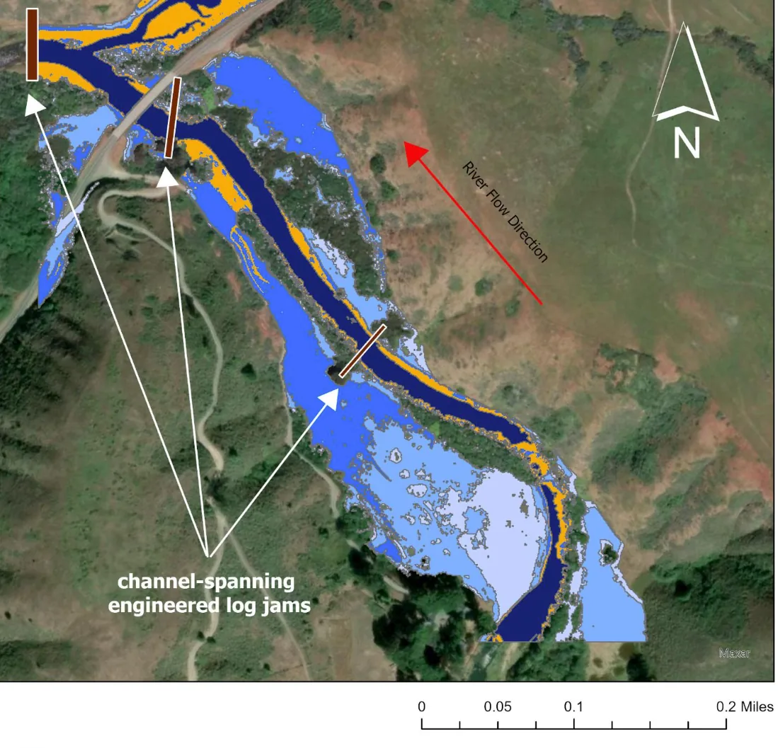
The elevation data is 2018 USGS 3DEP LiDAR at QL2, pulled from OpenTopography. I spot-checked the point cloud in FUSION before committing to the download and got a first-return density of about 7.2 points per square meter, which is enough to resolve the low ground I was after. Ground classification is where it stopped cooperating. FUSION’s ground filter kept exiting on me, probably something in the LAS headers, so I rewrote the headers with las2las and classified ground in LAStools with lasground_new instead. From the ground returns I built a 1 m bare-earth DEM in FUSION with gridsurfacecreate, exported it to ASCII, and took it into ArcGIS Pro. There I added a hillshade and used the raster calculator to cut masks at 1 m, 2.5 m, 3 m and 3.5 m above the current water surface, then converted each mask to polygons so I could get an area for every band.
What I learned
Two things, and the first one is that a tool failing is not a result. FUSION’s ground filter quitting cost me the afternoon, and the fix was to stop trying to make it work and classify in LAStools instead, which is a decision you can only make once you stop treating the software as the method. The second is about scale. Getting the water up two meters is aggressive, and the alternative of excavating for it comes to roughly 44,230 cubic yards, which is around 550 backyard pools of material. Putting the number in pools is what made it obvious it wasn’t happening. A volume in cubic yards is a number. A volume in swimming pools is an answer.
Results, in the source’s own terms
Band heights are measured against bank-full water surface under normal, non-storm conditions. To widen the stream by anything meaningful for salmon, the water has to come up at least two meters, which is the gold band on the map. Storms may do it on their own, and log jams are the cheap durable way to do it on purpose. The catch is that a two-meter design head can become a four-meter rise in a storm and put the nearby road under water. So the honest reading is a compromise. Smaller cut channels, or log jams plus something done about the road.
Nobody acted on this
Honest limits
- This was coursework. The Marin Resource Conservation District and the Marin Agricultural Land Trust are cited in it because their work is the reason the site is interesting, not because either of them commissioned or saw any of this.