Class assignment · Fuzzy overlay in ArcGIS · Published December 2025
Modeling methane potential in an alpine floodplain
Five things that have to be true at once for a pixel to be worth sampling, and a map of where they are.
What it was
Methane comes out of wetland soils unevenly, and a lot of what drives that sits in microsites too small for any satellite to see. What you can model is the setting those microsites tend to sit in. So the project was a suitability model for a river floodplain near Crested Butte, Colorado, in the Slate River watershed. Not a prediction of flux, and not a substitute for going out and measuring. A map of where the conditions line up, so a future sampling trip knows where to start.
Where this sits relative to the thesis
This was a class project, and it’s the one that pointed me toward the thesis work. Same watershed, same reason for caring about it. It isn’t the thesis and it doesn’t share the thesis’s data or its numbers. It’s the earlier, coarser look that made the finer one worth doing.
How it worked
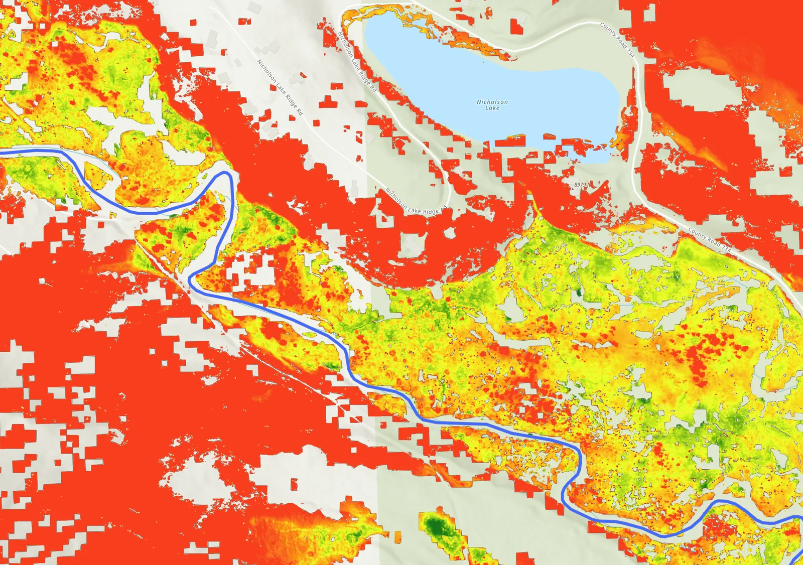
Deductive modeling, which means the drivers came from what is known to control methanogenesis rather than from fitting anything to observations. Five layers. Topographic wetness from a HAND surface, scoring hydrologic depressions high. A vegetation moisture index built from phenology residuals, scoring late-season greenness high because that tends to mean water underneath. Canopy height from NEON airborne LiDAR, scoring open scrub-shrub wetlands under 2 m high. Leaf carbon to nitrogen ratio from NEON hyperspectral, scoring nutrient-rich litter high. And distance to the river, which I got by digitizing the channel and running Euclidean distance off it. Every layer was converted to a fuzzy membership score from 0 for unsuitable to 1 for optimal, then combined with a fuzzy product operator.
What I learned
The product operator is the part I’d defend. Combining the five layers by multiplication means any single factor at zero takes the whole pixel to zero, so the model can’t average its way past a missing requirement the way a weighted sum would. That’s a real claim about how the system works, and putting it in the operator makes it visible instead of burying it in weights. The other thing worth saying is what fell out of the limiting factor analysis. Across the broader area, suitability is held down by coarse terrain and canopy structure. But within the sites that resemble where we already sampled, the vegetation moisture index is the binding constraint more than 90 percent of the time. It’s doing the work of telling similar-looking ground apart.
Nothing here was field-validated
Honest limits
- The model has not been checked against measured flux. Its own conclusion says what would have to happen next, which is a stratified sampling campaign to go and find out whether the high-suitability ground it flags actually produces methane. Until that happens this is a map of a hypothesis.